RavenDB 7.0 introduces vector search using the Hierarchical Navigable Small World (HNSW) algorithm, a graph-based approach for Approximate Nearest Neighbor search. HNSW enables efficient querying of large vector datasets but requires random access to the entire graph, making it memory-intensive.

HNSW's random read and insert operations demand in-memory processing. For example, inserting 100 new items into a graph of 1 million vectors scatters them randomly, with no efficient way to sort or optimize access patterns. That is in dramatic contrast to the usual algorithms we can employ (B+Tree, for example), which can greatly benefit from such optimizations.

Let’s assume that we deal with vectors of 768 dimensions, or 3KB each. If we have 30 million vectors, just the vector storage is going to take 90GB of memory. Inserts into the graph require us to do effective random reads (with no good way to tell what those would be in advance). Without sufficient memory, performance degrades significantly due to disk swapping.

The rule of thumb for HNSW is that you want at least 30% more memory than the vectors would take. In the case of 90GB of vectors, the minimum required memory is going to be 128GB.

Cost reduction

You can also use quantization (shrinking the size of the vector with some loss of accuracy). Going to binary quantization for the same dataset requires just 3GB of space to store the vectors. But there is a loss of accuracy (may be around 20% loss).

We tested RavenDB’s HNSW implementation on a 32 GB machine with a 120 GB vector index (and no quantization), simulating a scenario with four times more data than available memory.

This is an utterly invalid scenario, mind you. For that amount of data, you are expected to build the HNSW index on a machine with 192GB. But we wanted to see how far we could stress the system and what kind of results we would get here.

The initial implementation stalled due to excessive memory use and disk swapping, rendering it impractical. Basically, it ended up doing a page fault on each and every operation, and that stalled forward progress completely.

Optimization Approach

Optimizing for such an extreme scenario seemed futile, this is an invalid scenario almost by definition. But the idea is that improving this out-of-line scenario will also end up improving the performance for more reasonable setups.

When we analyzed the costs of HNSW in a severely memory-constrained environment, we found that there are two primary costs.

1. Distance computations: Comparing vectors (e.g., cosine similarity) is computationally expensive.
2. Random vector access: Loading vectors from disk in a random pattern is slow when memory is insufficient.

Distance computation is doing math on two 3KB vectors, and on a large graph (tens of millions), you’ll typically need to run between 500 - 1,500 distance comparisons. To give some context, adding an item to a B+Tree of the same size will have fewer than twenty comparisons (and highly localized ones, at that).

That means reading about 2MB of data per insert on average. Even if everything is in memory, you are going to be paying a significant cost here in CPU cycles. If the data does not reside in memory, you have to fetch it (and it isn’t as neat as having a single 2MB range to read, it is scattered all over the place, and you need to traverse the graph in order to find what you need to read).

To address this issue, we completely restructured how we go about inserting nodes into the graph. We avoid serial execution and instead spawn multiple insert processes at the same time. Interestingly enough, we are single-threaded in this regard. We extract from the process the parts where it does the distance computation and loads the vectors.

Each process will run the algorithm until it reaches the stage where it needs to run distance computation on some vectors. In that case, it will yield to another process and let it run. We keep doing this until we have no more runnable processes to execute.

We can then scan the list of nodes that we need to process (run distance computation on all their edges), and we can then:

• Gather all vectors needed for graph traversal.
• Preload them from disk efficiently.
• Run distance computations across multiple threads simultaneously.

The idea here is that we save time by preloading data efficiently. Once the data is loaded, we throw all the distance computations per node to the thread pool. As soon as any of those distance computations are done, we resume the stalled process for it.

The idea is that at any given point in time, we have processes moving forward or we are preloading from the disk, while at the same time we have background threads running to compute distances.

This allows us to make maximum use of the hardware. Here is what this looks like midway through the process:

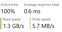
As you can see, we still have to go to the disk a lot (no way around that with a working set of 120GB on a 32GB machine), but we are able to make use of that efficiently. We always have forward progress instead of just waiting.

Don’ttry this on the cloud - most cloud instances have a limited amount of IOPS to use, and this approach will burn through any amount you have quickly. We are talking about roughly 15K - 20K IOPS on a sustained basis. This is meant for testing in adverse conditions, on hardware that is utterly unsuitable for the task at hand. A machine with the proper amount of memory will not have to deal with this issue.

While still slow on a 32 GB machine due to disk reliance, this approach completed indexing 120 GB of vectors in about 38 hours (average rate of 255 vectors/sec). To compare, when we ran the same thing on a 64GB machine, we were able to complete the indexing process in just over 14 hours (average rate of 694 vectors/sec).

Accuracy of the results

When inserting many nodes in parallel to the graph, we risk a loss of accuracy. When we insert them one at a time, nodes that are close together will naturally be linked to one another. But when running them in parallel, we may “miss” those relations because the two nodes aren’t yet discoverable.

To mitigate that scenario, we preemptively link all the in-flight nodes to each other, then run the rest of the algorithm. If they are not close to one another, these edges will be pruned. It turns out that this behavior actually increased the overall accuracy (by about 1%) compared to the previous behavior. This is likely because items that are added at the same time are naturally linked to one another.

Results

On smaller datasets (“merely” hundreds of thousands of vectors) that fit in memory, the optimizations reduced indexing time by 44%! That is mostly because we now operate in parallel and have more optimized I/O behavior.

We are quite a bit faster, we are (slightly) more accurate, and we also have reasonable behavior when we exceed the system limits.

        What about binary quantization?

I mentioned that binary quantization can massively reduce the amount of space required for vector search. We also ran tests with the same dataset using binary quantization. The total size of all the vectors was around 3GB, and the total index size (including all the graph nodes, etc.) was around 18 GB. That took under 5 hours to index on the same 32GB machine.

If you care to know what it is that we are doing, take a look at the Hnsw.Parallel file inside the repository. The implementation is quite involved, but I’m really proud of how it turned out in the end.